3 Data
3.1 Overview
This chapter presents the datasets and data cleaning processes that are common between the proceeding analysis chapters.
3.2 Geographies of England
This thesis is concerned only with England, as Scotland, Wales, and Northern Ireland each have their own separate deprivation data which are not comparable. The geographies in England form a nested hierarchy of spatial units from regions to districts to Middle-layer Super Output Areas (MSOAs) to Lower-layer Super Output Areas (LSOAs). The number of units for each geography are summarised in Table 3.1.
| Geography | Number of units | Median (5\(^{\text{th}}\)-95\(^{\text{th}}\) percentile) population in 2019 |
|---|---|---|
| region | 9 | 5,934,037 (3,536,336-9,092,877) |
| district | 314 | 140,271 (68,238-380,483) |
| MSOA | 6791 | 7985 (5760–11,917) |
| LSOA | 32,844 | 1620 (1235-2468) |
England is divided into nine regions (North East, North West, Yorkshire and the Humber, East Midlands, West Midlands, East of England, South East, South West, London). Within these regions, there are 314 local authority districts. Districts are administrative geographies formed from a mixture of London boroughs, metropolitan and non-metropolitan districts, and unitary authorities. They are responsible for local policies, and are therefore subject to local government restructuring and boundary changes. To ensure geographic consistency, all data were mapped to the district boundaries from 2020.
Output Areas (OAs) are the smallest building block for spatial census statistics, with between 40 and 250 households and typically 100 to 625 people, and are designed to have some socioeconomic homogeneity. LSOAs are a type of census geography made up of around four or five OAs. MSOAs are then composed of around four or five LSOAs, and these MSOAs fit within district boundaries. OAs, LSOAs, and MSOAs are all statistical units which are designed by the Office for National Statistics (ONS) purely for analysis purposes, so researchers can use spatial units with similar, but small, population sizes. No policies are created using these boundaries (Office for National Statistics, 2022a). Again, for geographic consistency, all data were mapped to the output area hierarchy from the 2011 census.
3.3 Data sources
3.3.1 Deaths
This thesis is primarily concerned with modelling death rates for small areas in England. This requires two data sources: counts of deaths, and population counts. The counts of deaths come from de-identified civil registration data for all deaths in England from 2002 to 2019. In other words, every death in England from 2002 to 2019.
The data is extracted from the ONS database and held by SAHSU in a secure environment as individual death records are identifiable data. The data are updated every year and are mostly complete for previous years, but a handful of deaths are registered in later extracts if the ONS have been waiting on a coroner’s report to identify the underlying cause of death.
Each record comes with information on postcode of residence, allowing us to assign each death into a spatial unit for analysis. For each analysis, deaths were stratified into the following age groups: 0, 1–4, 5–9, 10–14, then 5-year age groups up to 80–84, and 85 years and older. There are also a series of ICD-10 (International Classification of Diseases, Tenth Revision) codes from the death certificate associated with the underlying and contributory causes leading to the death. Here, I focus only on the underlying cause of death, which has been assigned using selection algorithms to improve consistency between doctors (Office for National Statistics, 2022b).
3.3.2 Population
The second data source we require are population counts. These are taken from mid-year population estimates of the usual resident population by the ONS (Office for National Statistics, 2021a, 2021b). The ONS estimates inter-censal populations on a rolling basis, updating the previous year’s value using the change in the population in GP patient registration data as an indicator of the true population change. The LSOA populations are fully consistent with estimates for higher levels in the nested geographical hierarchical including MSOAs, districts, regions and the national total for England (Office for National Statistics, 2021c).
3.3.3 Community deprivation
I used data for the following measures of socioeconomic deprivation from the English Indices of Deprivation:
- Income deprivation (also referred to as poverty). The proportion of the geographical population claiming income-related benefits due to being out of work or having low earnings.
- Employment deprivation (also referred to as unemployment). The proportion of the relevant population of the geography involuntarily excluded from the labour market due to unemployment, sickness or disability, or caring responsibilities.
- Education, skills and training deprivation (also referred to as low education). Lack of attainment and skills, including education attainment levels, school attendance, and language proficiency indicators in the geographical population.
The above measures are the three largest contributors to the Index of Multiple Deprivation (IMD), excluding a domain on health that also uses mortality data. The data are produced at the LSOA level (Ministry of Housing, Communities & Local Government, 2019).
IMD data are not available for every year. The analysis period for the thesis is 2002 to 2019, so I used data for these measures for 2004, as data for 2002 were not available, and 2019. The 2004 data on deprivation domains were reported for LSOA boundaries from the 2001 census. I mapped these data to the 2011 census LSOA boundaries by assigning the 2001 LSOA score to all postcodes contained within it, then overlaying the 2011 LSOA boundaries, and averaging the score for all constituent postcodes of each LSOA, to obtain the corresponding score for each 2011 LSOA.
The definition of the indicators can change over time. Further, the indicator used for measuring education, skills and training deprivation (low education) is not directly interpretable because it combines multiple concepts and cannot be simply expressed as a proportion of the population. Therefore, I used ranking rather than scores so that comparisons can be made not only across spatial units in a single year, but also across the different years.
The deprivation data for geographies larger than LSOAs in Table 3.1 were created by ranking the population-weighted average of scores for all constituent LSOAs, as done previously for districts (Ministry of Housing, Communities & Local Government, 2019).
3.3.4 Migration
I also used estimates of population turnover, defined as the proportion of households in each LSOA in 2019 who were different from those who had lived there in 2002, from the Consumer Data Research Centre. The Consumer Data Research Centre estimates these proportions by using the names of households members, individually and in combination, and addresses and dates of records from electoral and consumer registers and land registry sales data (van Dijk et al., 2021). Estimates of population turnover for MSOAs were created by taking the mean across all constituent LSOAs (Ministry of Housing, Communities & Local Government, 2019).
3.4 Exploratory data analysis
Before fitting any models, I explored the data visually, in this case looking at how total mortality varies over different cross sections: sex, age, space, time.
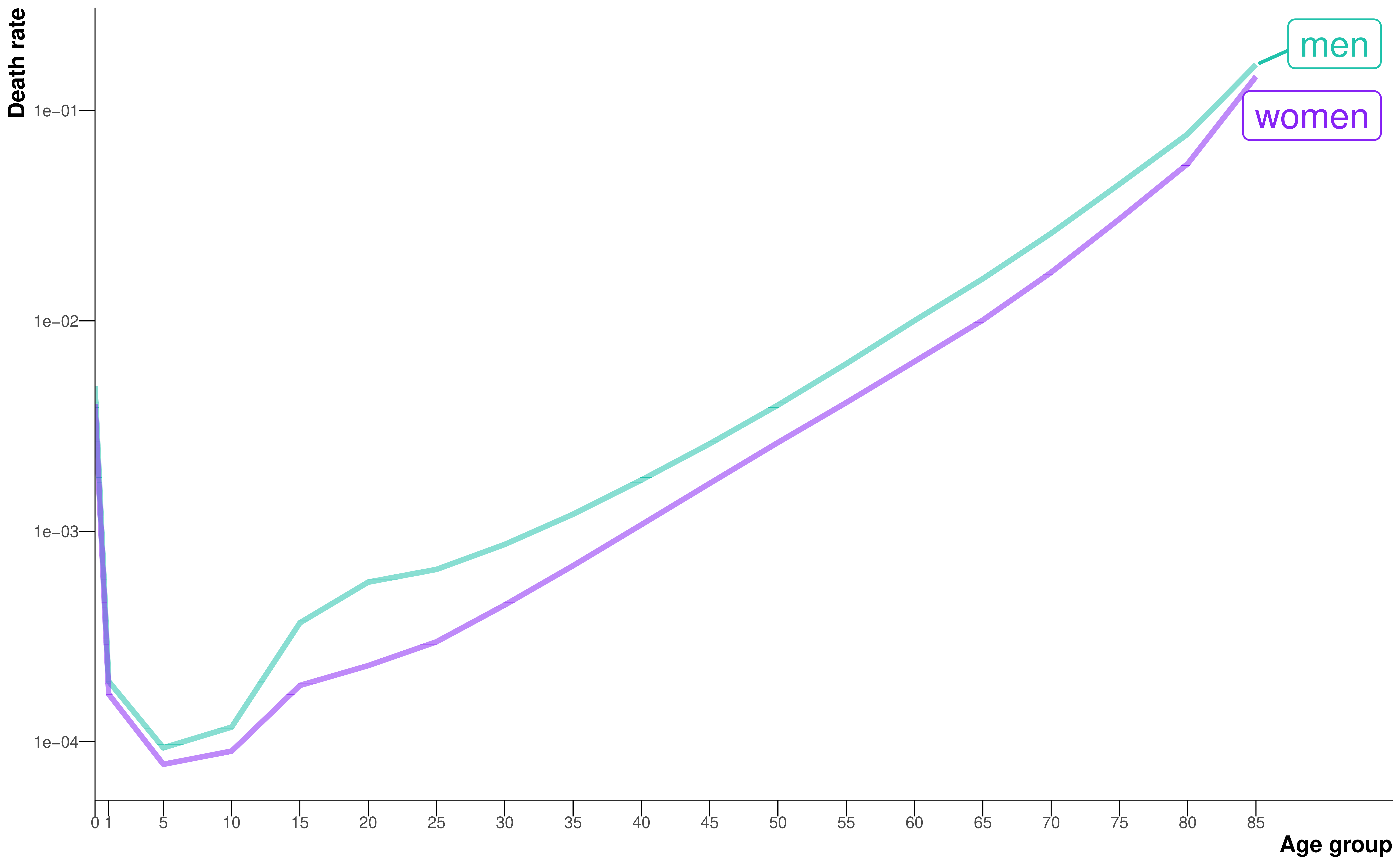
The general age pattern, after aggregating all years and separating into age groups, follows a J-shape curve, with raised infant and older age mortality (Figure 3.1). Male mortality is higher at all ages, but particularly in young adulthood (15-29 years) due to injuries resulting from risky behaviours.
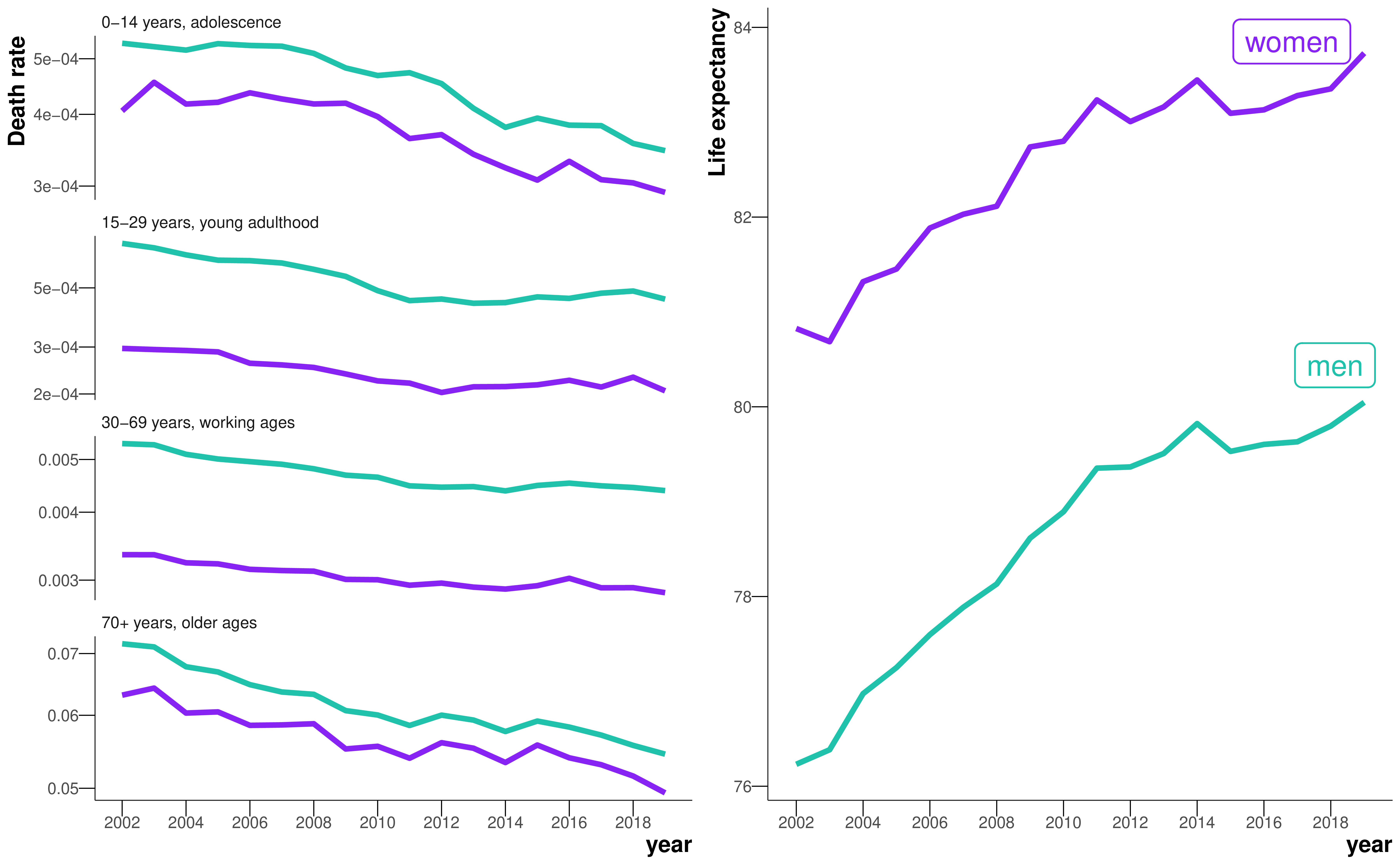
Figure 3.2 looks at the trends over time for wider age groups. I did not use the 5-year age groups because the number of deaths for certain age groups at single years were small, and any data presented should be non-disclosive in accordance with SAHSU’s data sharing agreement. In general, death rates have decreased from 2002 to 2019 in all age groups, but with slowing progress in young adulthood and working ages (30-69 years). Likewise, life expectancy has improved throughout the study period, but has stalled since around 2010 for both sexes.
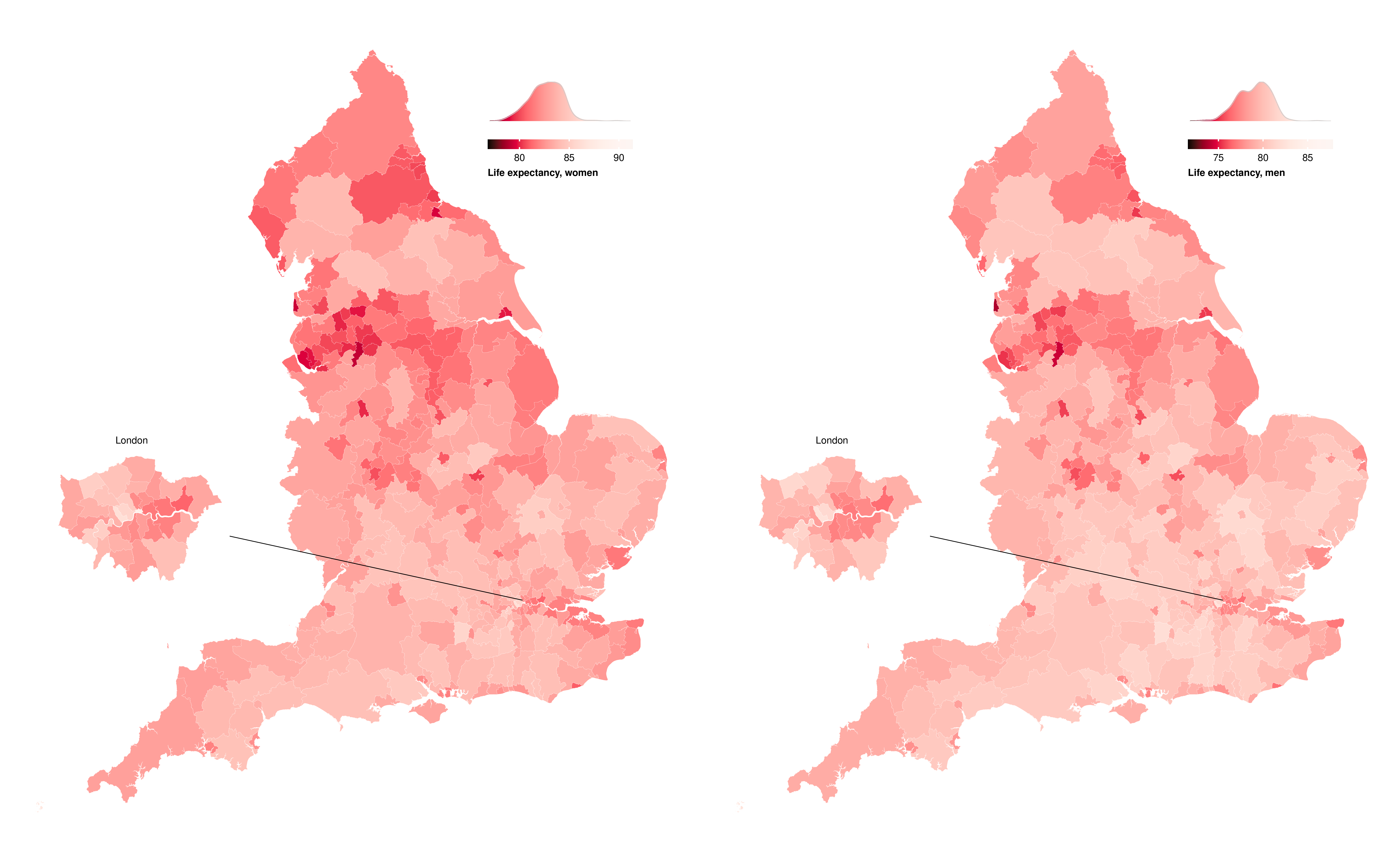
Figure 3.3 shows the geography of life expectancy after aggregating deaths over the entire study period by district. For both sexes, the picture is similar: pockets of low life expectancy in the urban North West, North East, and West Midlands.
In this section, I have taken slices across each dimension, but the aim in the following chapters is to calculate death rates for each sex-age-space-time stratum.
3.5 Summary
All-cause and cause-specific mortality estimates require data on deaths and populations. Individual death records with information of sex, age at death, cause of death, year of death, and place of residence have been taken from the ONS database and held by SAHSU in a secure environment. I have used small-area population estimates created by the ONS. I also introduced datasets on area-level deprivation and migration which will be used to put mortality estimates into context.