state space model

A state space model is a partially observed Markov model:

• are the latent states
• are the observations
• are exogenous inputs

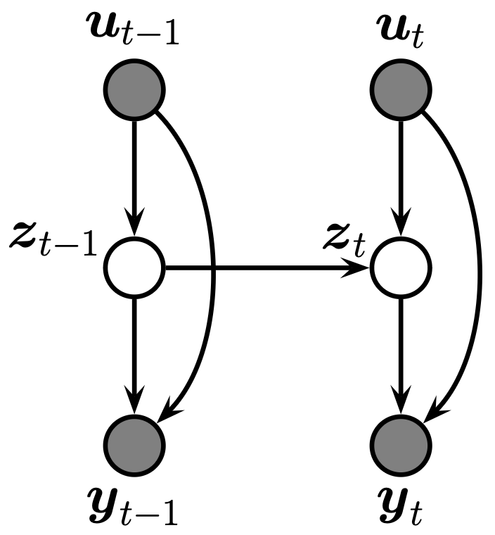
Using the Markov property, the above probabilistic graphical model forms the joint distribution

Dynamics model	Observation model	Model
Categorical (discrete states)	Any	[[./hidden markov model
Linear Gaussian	Linear Gaussian	[[./linear gaussian ssm
Nonlinear, Gaussian noise	Nonlinear, Gaussian noise	[[./nonlinear gaussian ssm
Gaussian (linear or nonlinear)	Non-Gaussian	[[./generalised gaussian ssm
Continuous-time SDE	Discrete-time observations	[[./continuous-discrete state space model

See ssm resources.

Inference and parameter estimation

Inference has two parts: an inner loop (state estimation given fixed ) and an outer loop (learning using the inner loop’s log marginal likelihood ).

State estimation (inner loop)

• Filtering: — online, forward pass
• Smoothing: — offline, forward-backward

	HMM	LGSSM	Nonlinear Gaussian	Generalised
Discrete filter	Exact	—	—	—
Kalman filter	—	Exact	—	—
EKF / UKF	—	Overkill	Approximate	Poor*
Particle filter (SMC)	Overkill	Overkill	Yes	Yes

*Local Gaussian approximation of non-Gaussian likelihoods (e.g. CMGF) may be poor for multimodal or heavy-tailed distributions.

Parameter estimation (outer loop)

• MLE / MAP: differentiate w.r.t. , optimise with gradient ascent (e.g. optax)
• MCMC: sample using the inner loop likelihood. For non-Gaussian models, a particle filter gives a noisy but unbiased likelihood estimate that still targets the correct posterior (Particle MCMC). Use with e.g. blackjax or numpyro
• EM: E-step runs filter + smoother for expected sufficient statistics; M-step updates

Model and inference are decoupled — dynamax bundles them together; cuthbert keeps them separate.