polar coordinates

Curvilinear coordinate systems for axial and radial symmetry.

---

cylindrical polar coordinates

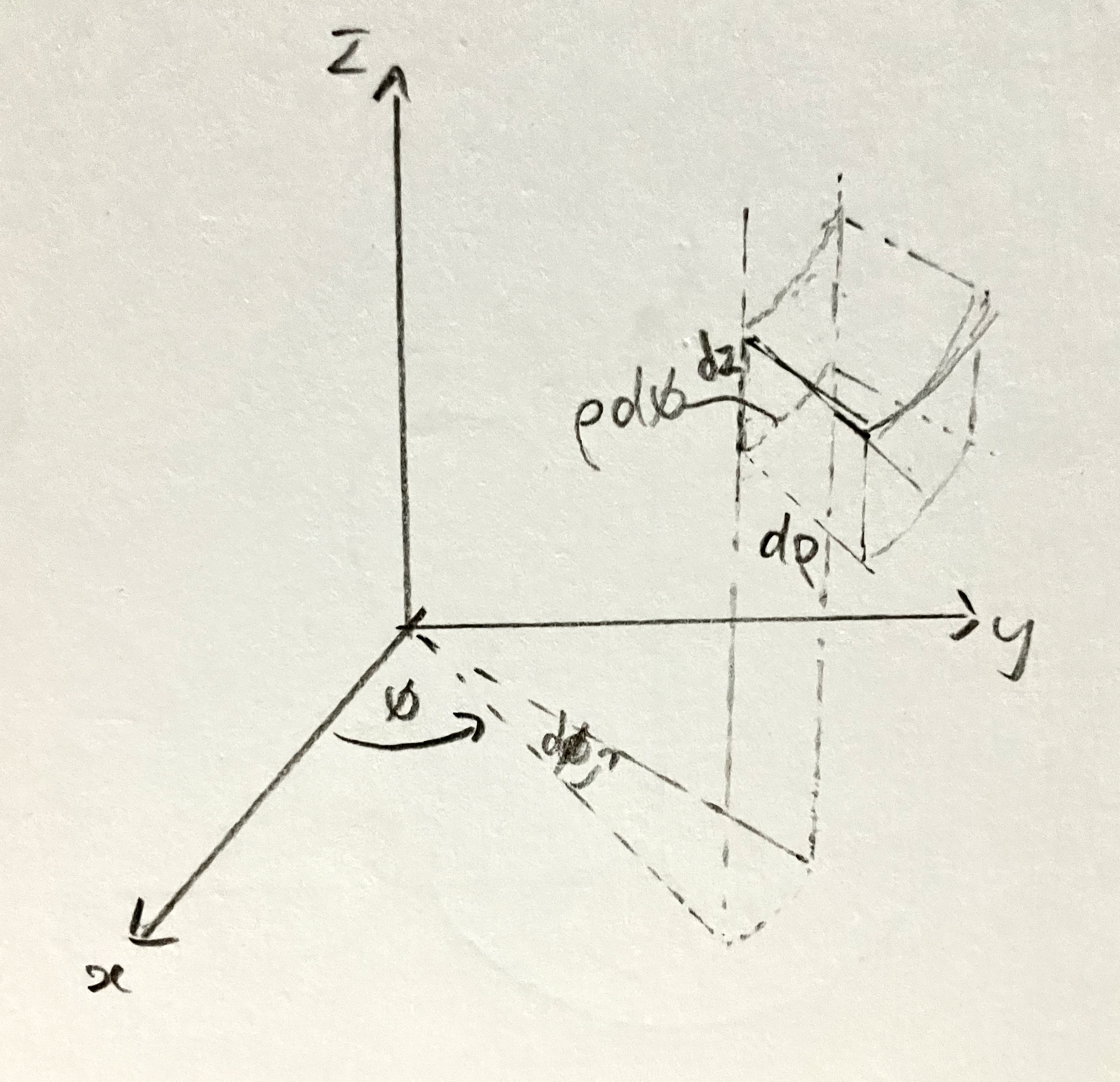
transformation

Basis vectors (position-dependent — , rotate with ):

line element & scale factors

Jacobian & volume element

Equivalently .

J = jnp.linalg.det(jax.jacfwd(cylindrical_to_cartesian)((ρ, φ, z)))  # = ρ

operators

From , matching with chain rule :

General curvilinear divergence :

Curl from the curvilinear determinant :

Laplacian :

---

spherical polar coordinates

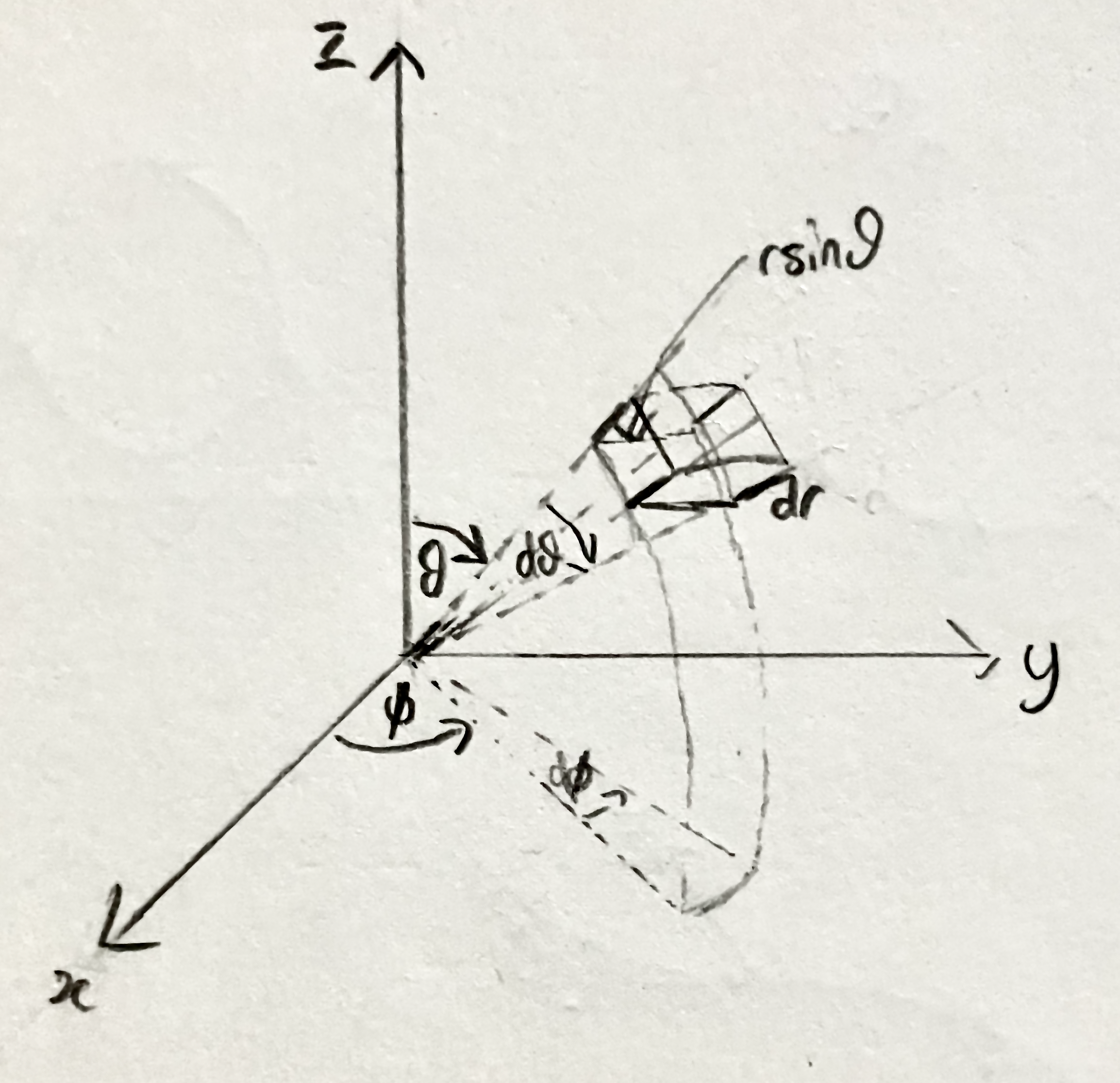
transformation

Basis vectors:

line element & scale factors

Jacobian & volume element

Equivalently .

J = jnp.linalg.det(jax.jacfwd(spherical_to_cartesian)((r, θ, φ)))  # = r² sin θ

operators

From , matching with chain rule :

General curvilinear divergence :

Curl from the curvilinear determinant :

Laplacian :

The radial part can also be written , useful for Laplace’s equation.

# gradient in curvilinear via composite function
df_dcoords = jax.grad(lambda c: f_cartesian(*cylindrical_to_cartesian(*c)))((ρ, φ, z))
grad_physical = df_dcoords / jnp.array([1., ρ, 1.])  # divide by h_i
 
# vector Laplacian in Cartesian (avoid curvilinear operators):
lap_A = lambda x: jnp.array([jnp.trace(jax.hessian(lambda x: A(x)[i])(x))
                              for i in range(3)])